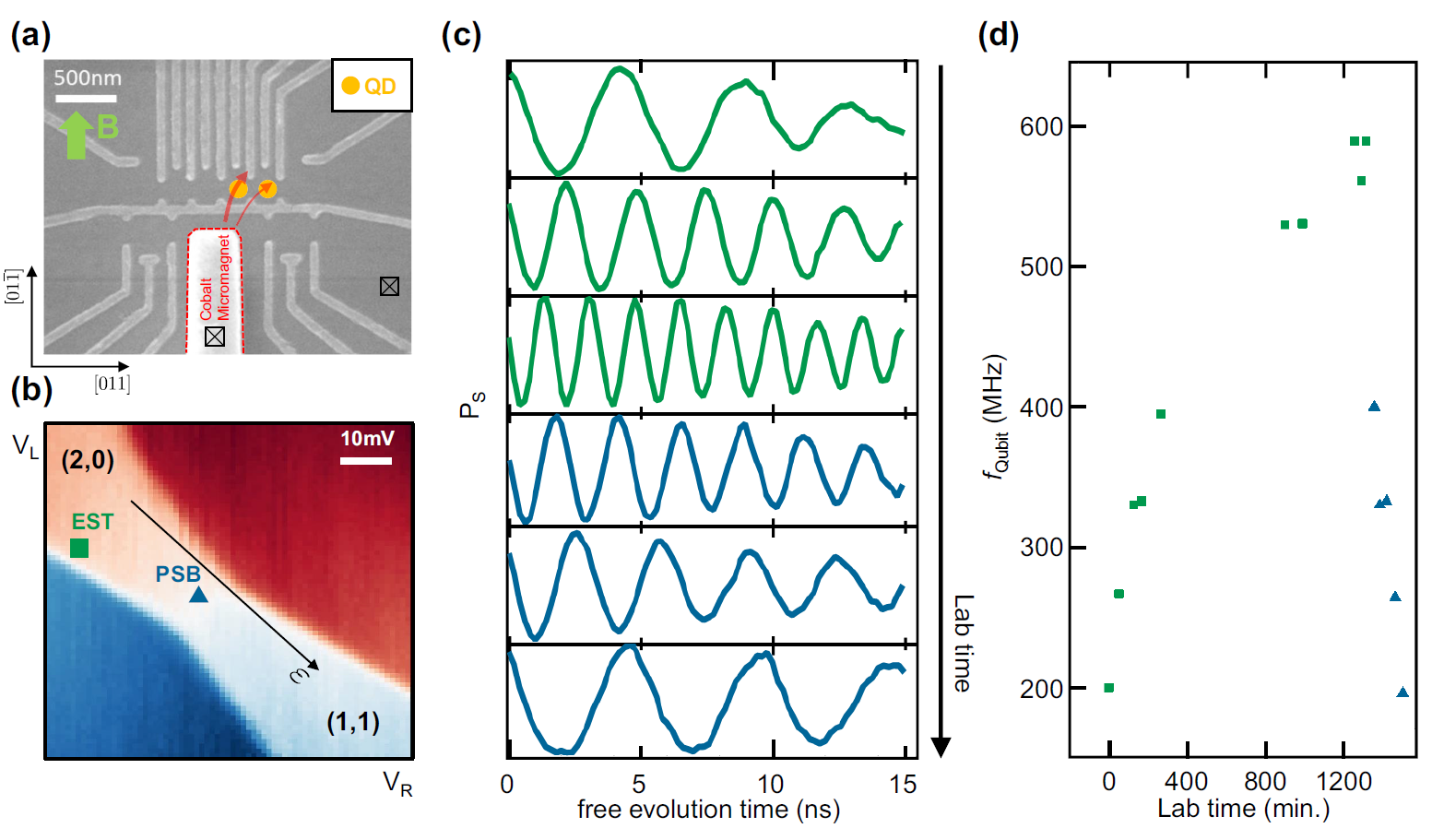
Figure 1 | Bidirectional Dynamic Nuclear Polarization Controlled by Pulse Parking Position (a) The AlGaAs/GaAs quantum dot device used throughout the experiment, whose crystallographic alignment is indicated at the lower-left corner. The orange circle marks the location of the quantum dot, and the crossed boxes indicate ohmic contacts. The cobalt micromagnet is enclosed by the red dotted lines, whose field direction is qualitatively plotted by the red transparent arrow. The magnetic field is applied in-plane to the 2DEG, as depicted in the upper left corner. (b) The charge stability diagram near (1,1) and (2,0) regimes. The location of the EST (PSB) regime is marked by the green box (blue triangle). (c) The Rabi oscillation, which is plotted after a series of Rabi pulse applications whose parking position was at either EST (green) or PSB (blue). When parked at EST, the oscillation frequency increased with the lab time, indicating that the serial Rabi pulse application increased ∆Bz. On the contrary, the parking at PSB showed the exact opposite behavior. (d) The change of the Rabi oscillation frequency as a function of lab time. The PSB- and EST-parking scheme shows the opposite behavior.
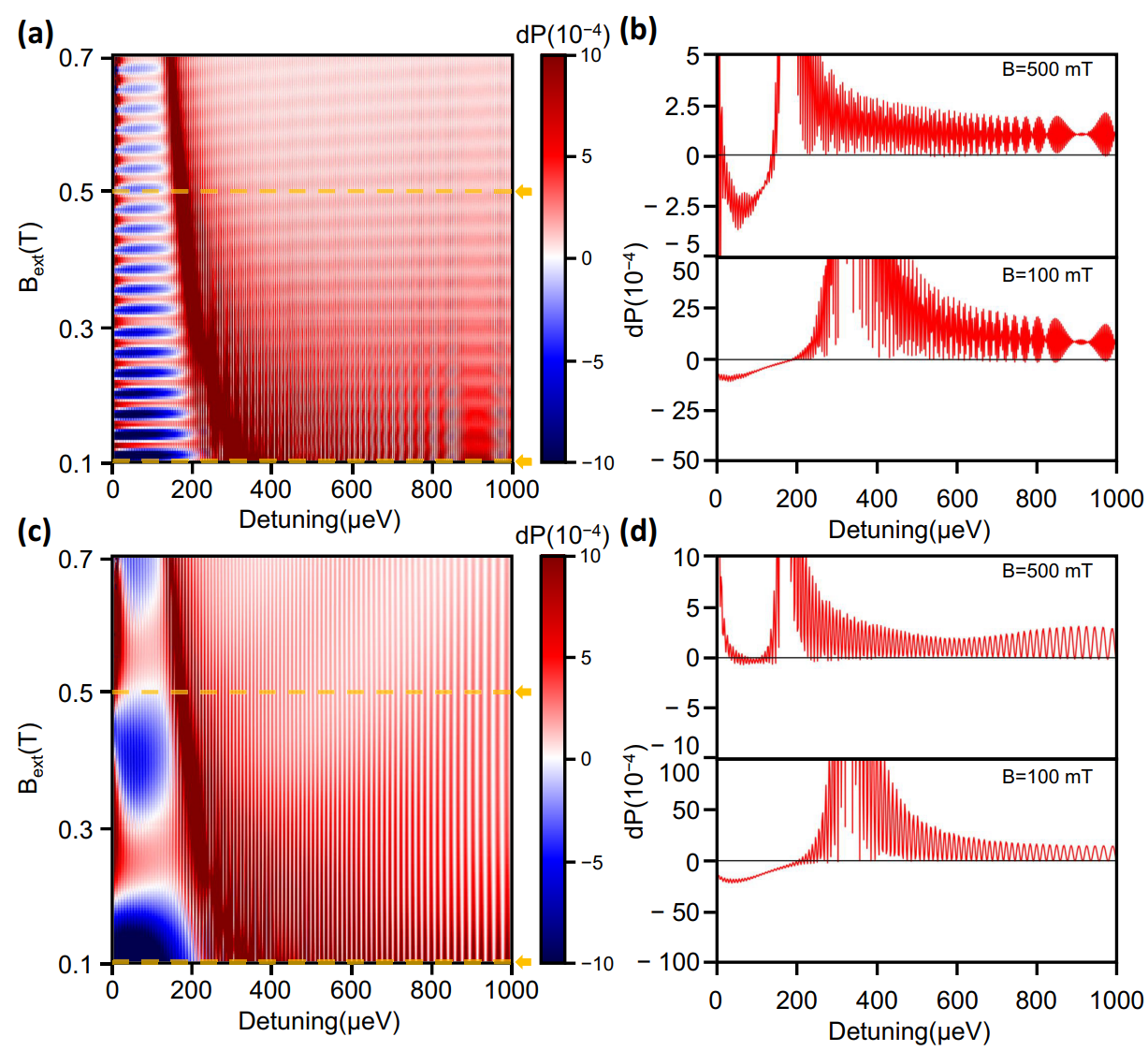
Figure 2 | Analysis of Triplet State Dynamics Under a Single Rabi Pulse (a) The color plot of dP change under a single Rabi pulse. The clear reversal appears. The orange dotted lines mark the location for the left line-cut plot. (b) The line-cut plot of (a). Neither of line-cut shows dP reversal, indicating that T(2, 0) included dynamics is crucial in the T+ pumping effect in PSB regime. (c) The color plot of dP change under a single Rabi pulse with zero pulse width. The orange dotted lines mark the location for the left line-cut plot. (d) The line-cut of Fig (c).
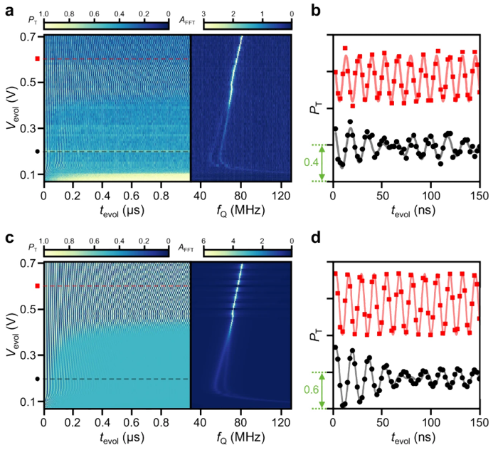
Figure 3 | Comparison of Experimental Data and Numerical Simulation of Qubit Dynamics (a) Experimental Ramsey oscillations of a singlet-triplet qubit in a 28Si/SiGe device as a function of evolution time (tevol) and gate voltage (Vevol). The FFT result (right) shows a characteristic peak splitting below Vevol ≈ 0.42 V. (b) Line cuts of the experimental data at two different voltages. The bottom trace clearly shows a "beating" pattern, which is a signature of coherent coupling to a neighboring quantum dot spin states. (c) Numerical simulation of the Ramsey oscillations based on a quantum master equation with a dephasing Lindbladian. The simulation consistently reproduces the significant decoherence and FFT peak splitting observed in the experiment. (d) Simulated line cuts that successfully replicate the experimental data, including the characteristic beating of the oscillation in the strong coupling regime.
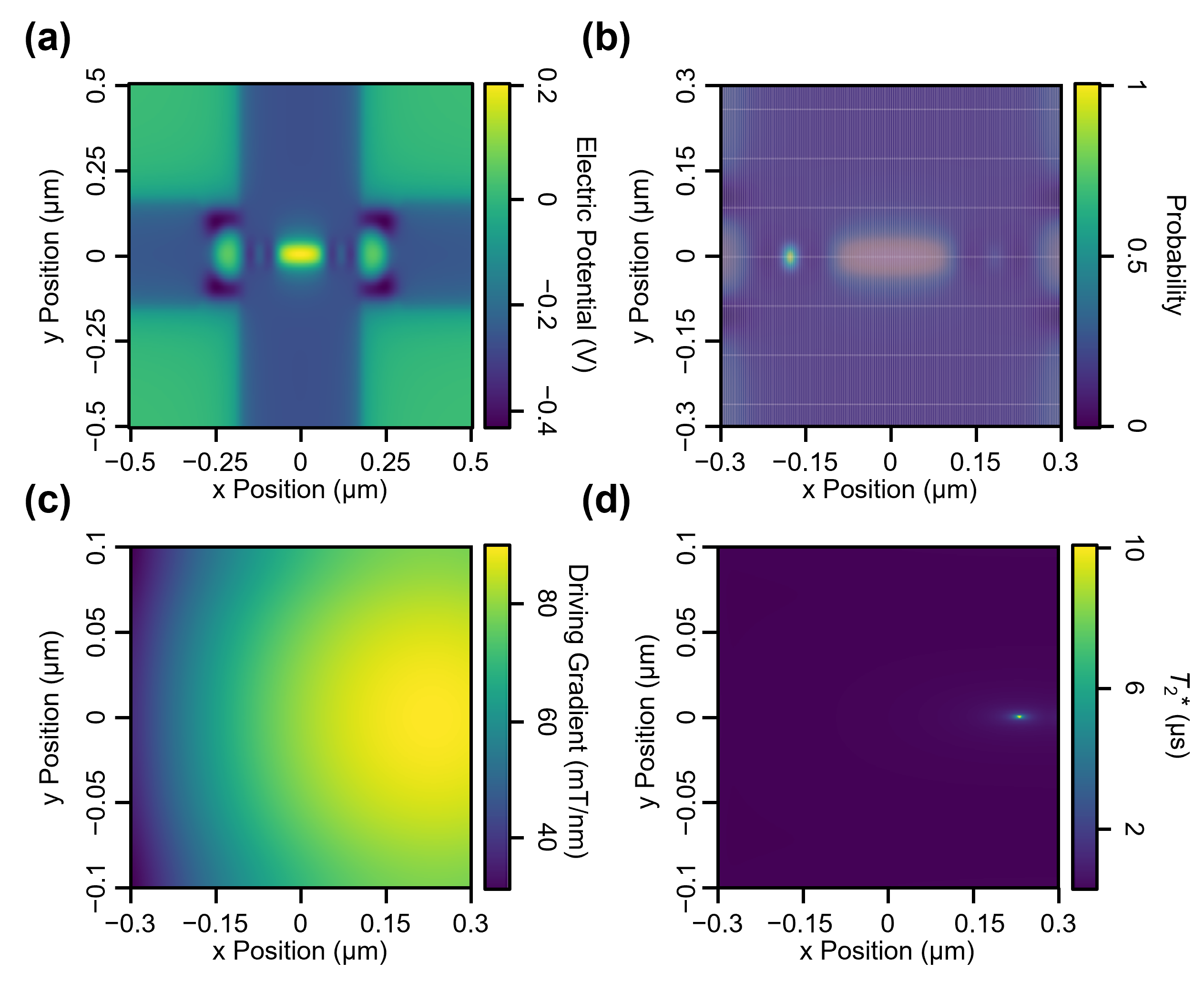
Figure 4 | End-to-End Simulation Pipeline from Device Geometry to Qubit Performance (a) The 2D electrostatic potential landscape of a double quantum dot, calculated from the device's CAD geometry using a Green's function-based approximation. (b) The ground state probability density of a single electron, obtained by solving the 2D Schrödinger equation with the potential from (a) using a finite difference method. (c) The effective magnetic driving gradient experienced by the electron. This is calculated by convolving the micromagnet's simulated stray field with the electron probability density from (b). (d) The final calculated map of the qubit's dephasing time (T2*). The "sweet spot" of long coherence is determined from the effective magnetic field, providing a direct link between device design and qubit performance.
Quantum Dot Spin Qubit Experiments Jun. 2020 – Jun. 2025
⌜Developed comprehensive simulation frameworks to model complex quantum phenomena in semiconductor qubits. Created a full, end-to-end simulation package that computes electron wavefunctions from CAD layouts by solving the Schrödinger equation, and convolves them with MuMax3-simulated magnetic fields. Utilized QuTiP to solve the quantum master equation with Lindblad operators to reproduce experimental observations of qubit-environment interactions in silicon. Modeled dynamic nuclear polarization in GaAs dots using a modified Hubbard model.⌟
To complement my experimental work, I have developed a strong expertise in computational modeling to understand the complex physics governing quantum dot systems.
My initial work focused on explaining the bidirectional dynamic nuclear polarization (DNP) observed in GaAs singlet-triplet qubits.
By modeling the system with a modified Hubbard model that incorporated excited-level spin mixing, my simulation successfully reproduced the experimental DNP behavior, providing a theoretical explanation for this previously unexplained phenomenon.
The details can be found in my Master's thesis.
Building on this experience, I later used the QuTiP (Quantum Toolbox in Python) framework to investigate the coherent interaction between a singlet-triplet qubit and a neighboring multi-electron quantum dot in a 28Si/SiGe device.
To explain the characteristic beating and dephasing observed in Ramsey measurements (as seen in Figs. 2c and 3c of our npj Quantum Information publication),
I solved the quantum master equation for the coupled system, introducing a phenomenological Lindbladian for dephasing.
These computationally intensive simulations were accelerated by leveraging Python's multiprocessing capabilities to parallelize the calculations.
Most recently, to investigate an anomalously long coherence time observed in a silicon device, I developed a full, end-to-end simulation package that connects device geometry to quantum mechanical properties.
This package features a pipeline that: (1) Parses device layouts from CAD files using a custom Python tool, (2) Calculates the 2D electrostatic potential landscape, (3) Solves the 2D Schrödinger equation using a Finite Difference Method to obtain the electron wavefunction, (4) Simulates the micromagnet's 3D stray field using MuMax3, and finally, (5) Convolves the wavefunction with the stray field to compute the effective magnetic field experienced by the qubit.
To accelerate this computationally intensive step, the core calculation was implemented in C++ utilizing multithreading, which achieved a nearly 100x speedup compared to a pure Python implementation. This high-performance C++ backend was then seamlessly integrated into the Python workflow using Pybind11.
This tool, some of which can be found at this link, enables rapid design validation and a deeper understanding of the physics underlying our experimental results.